Personal Notes about The Definitive Guide to DAX
Disclaimer: this will be a long, long post, written in my own way. It’s essentially a dump of my personal notes, taken when reading “The Definitive Guide to DAX” written by Alberto Ferrari and Marco Russo. At my new workplace I’m going to use PowerBI and DAX a lot, thus my boss suggested me to read the book.
Yep, it is big and very technical, with 700+ pages rich in contents, but trust me, that’s the “Bible”, a must-read for anyone willing to work with PowerBI and DAX. There’s everything you need, from the basics commands to the most advanced functions, with complex topics such as context transition, query plan, and storage engine. Many examples, in addition, apart from explaining every concept introduced in the book (which focuses a lot on giving clear, practical explanations) explore edge cases that gave me lots of headaches in the past. Further examples and insights can be found on the authors’ site SQLBI.
It took me several weeks for finishing it, but I felt extremely prepared after the experience and grateful for such a useful resource that will be fundamental in my future. The authors did a terrific job and I am happy to support them and share a positive feedback of their work on my blog. Knowing that my memory is terrible I took accurate notes of everything I found interesting and what I have to read again. I hope it will help you as well!
My personal classification of each chapter
⚠️ VERY IMPORTANT, read it several times and understand everything
🔄 To read again, plenty of examples/documentation
✨ Useful
❓ Minor insights
1 ✨ What is DAX?
Introductive chapter that introduces the concept of Data Analysis eXpressions, there’s nothing more to add. There’s an interesting presentation of all the different points of view of possible users (the ones who come from an Excel Background, or a PowerBI one, a SQL one…). Personally, I felt in synthony with the ‘typical’ SQL user: learning that the FILTER DAX clause is the equivalent of a WHERE immediately cleared some doubts I had.
2 🔄 Introducing DAX
Very important section for beginners, explaining the most common functions and the difference between calculated column and measure.
It introduces the different data types, which are the classic ones (Integer, Float, Currency, Datetime, Boolean, Strings, Binary), with just a new type, Variant, which is DAX-specific and simply means that there could be different data types (such as Anyin Python).
There are brief introductions of the operators: arithmetic (+-*/), comparatives (<,>,=,<>,≥,≤), logic (&&, ||, IN, NOT) and tables, created with {} and must include parenthesis in case of multiple values. E.g. Colours = {”Red”, “White”, “Blue”}. Animals = {(”Dog”, “Woof”),( “Cat”, “Meow”)}
Calculated Columns
Written as ‘Table Name’[Column Name], calculated columns are new columns added to the data model, and you can use them just like a default one, independently from the context. Just be aware that in Import Mode (the standard one), they are calculated during the data refresh, then stored in memory, occupying some precious RAM! If you have a complex formula, don’t break it down into intermediate steps as you do in Excel, but rather create and test it in DAX Studio and store the result in a single calculated column to optimize the model.
You should use a calculated column if:
- The result will be in a slicer, matrix, pivot, or
FILTERcondition - You have an expression that is relative to the single row and doesn’t require aggregation, like
Price * Quantitywhich must use the Price of the row and the Quantity of the row - You have to categorize text or numbers, e.g. assigning a High, Medium, Low range, or 0-18, 18-25, 25+. Again, it’s when you don’t want to aggregate results
Measures
A measure is not directly associated with a table and it’s written as [Measure Name]. Generally, you should use them when you don’t want to calculate values for each row, but you want an aggregation: in fact, a measure has an implicit CALCULATE clause in its formula and is modified by the context (see Chapter 5). Here’s a good example:
If you create a calculated column like Sales[GrossMarginPct] = Sales[GrossMargin] / Sales[SalesAmount], you will see that the total is more than 100% (If our ten products have a 50% Gross Margin each, the table displays 50*10 → 500%)! DAX is applying the formula row-by-row, but we want to see the total instead. A measure GrossMarginPct := SUM ( Sales[GrossMargin] ) / SUM (Sales[SalesAmount] ) will give the correct result instead.
You should use a measure if:
- The value depends on the context and user’s selections
- Values are in an aggregate form
Variables
Write them at the beginning of the DAX formula as VAR TotalSales = SUM(Sales[SalesAmount]) ... RETURN *result (there must be a RETURN at the end). They are IMMUTABLE and generated at the start of the calculation. They are temporary measures existing only internally to the measure you are using, and they are very useful for breaking down a formula into more readable steps and for avoiding repetitions.
Basic Functions
Note: many of them have an iterative version (SUM/SUMX), these examples are the same:
Sales[DaysToDeliver] = INT ( Sales[Delivery Date] - Sales[Order Date] )
AvgDelivery := AVERAGE ( Sales[DaysToDeliver] )
// They are the same, but the second one is better optimized
AvgDelivery :=
AVERAGEX (
	Sales,
INT ( Sales[Delivery Date] - Sales[Order Date] ))- Basic:
SUM, AVERAGE, COUNT, COUNTBLANK, COUNTROWS, DISTINCTCOUNT, DISTINCTCOUNTNOBLANK - Logic:
AND, OR, IF, IFERROR, NOT, TRUE, SWITCH - Information:
ISBLANK, ISERROR, ISLOGICAL, ISNONTEXT, ISNUMBER, ISTEXT - Mathematical:
ABS, EXP, FACT, LN, LOG, LOG10, MOD, PI, POWER, QUOTIENT, SIGN, SQRT, RANDOM, RANDBETWEEN, ROUND, EVEN, ODDe many more - Textual:
CONCATENATE, CONCATENATEX, EXACT, FIND, FIXED, FORMAT, LEFT, LEN, LOWER, MID, REPLACE, REPT, RIGHT, SEARCH, SUBSTITUTE, TRIM, UPPER, VALUE - Conversions:
CURRENCY, INT, DATE, TIME, VALUE, DATEVALUE, FORMAT - Date & Time:
DATE, DATEVALUE, DAY, EDATE, EOMONTH, HOUR, MINUTE, MONTH, NOW, SECOND, TIME, TIMEVALUE, TODAY, WEEKDAY, WEEKNUM, YEAR, YEARFRAC - Relational:
RELATEDeRELATEDTABLE. They are very powerful, we will explore them later
3 ⚠️ Using basic table functions
FILTER
The book introduces FILTER and the EVALUATE concept, to be used on DAX Studio. With FILTER with multiple conditions, a good tip is to put the most restrictive at the top of the query, to optimize it in case of big tables.
ALL*
ALL* gets introduced too, they are extremely powerful: ALL, ALLEXCEPT, ALLCROSSFILTERED, ALLNOBLANKROW, ALLSELECTED. ALL IGNORES EVERY ACTIVE FILTER in the report and it’s useful when you calculate ratios and percentages compared to the total, regardless of filters and users’ selections. It returns a list of unique values, requiring a table or a list of columns, not an expression; if you use ALL with more than a column, it will give back all the possible unique combinations existing in the table. ALLEXCEPT can be translated as ‘take everything from that table except the following columns’. The rest will be explained in Chapter 14.
VALUES,DISTINCT,BLANK
Like ALL, VALUES and DISTINCT return a list of unique values too… With a big difference. VALUES returns the visible values, so it’s not ignoring the active filters, and the same does DISTINCT. They are different in the case of invalid relations. There’s a great example in the chapter: if, for example, a product is missing from the Product table, the join between it and the Sales table will have blank rows in the results. In this case, DISTINCT gets confused when calculating the average amount for product, while VALUES considers the blank row correctly in the division. TL;DR: use VALUES most of the cases.
There’s a brief insight about HASONEVALUE, a shortcut for IF ( COUNTROWS ( VALUES ( [colonna] ) ) = 1, VALUES ( [colonna] ); it has a second argument for returning a message if there’s more than a value: it can be useful for cards and elements that expect only one value to be selected.
4 ⚠️ Understanding Evaluation Context
⚠️️ The authors say that this chapter and #5 are the most important of the entire book. If you understand context, you will avoid the most common errors when you code in DAX. Read it several times until you understand everything!
In DAX, there are two completely different contexts impacting your formulas. Filter Context, which filters data, and Row Context, which iterates through tables. A context is, in short, the environment where the expression is evaluated.
Filter Context
I’m not able to explain it as well as in the book without examples, but here’s my personal interpretation.
Let’s take a table with a measure, say TotalSales = SUMX(Sales[Amount]. A table has rows and cells. Every expression is evaluated based on its cell, which in turn is modified based on active filters and the selected column. So, the TotalSales measure will be, say, 30Mln if I put it into a card with no filters and just a cell, but if I use it in a table with multiple rows the is split based on the row’s contents (imagine a division by Area: Europe, US, Asia → 30mln will become 10mln x 3 cells. Behind the scenes, DAX is adding a FILTER saying FILTER (Area = ‘Europe’) and so on, for every cell). So, the filter context changes the outcome of the expression considering the filters that become active if, for example, it’s inside a specific cell of a table. What’s important is the context of the cell containing it: which is precisely the filter context.
Row Context
The example I recommend to read carefully uses this calculated column Sales[Gross Margin] = Sales[Quantity] * ( Sales[Net Price] - Sales[Unit Cost] ). Now remember, this column reasons in terms of rows, so, how does DAX manages to understand which row is working on? Using row context, which is basically a cursor. Row context, then, calculates the expression by considering the row that contains it.
If you write Gross Margin as a measure, you lose the row context, thus you need the iterative version ending with X: Gross Margin := SUMX ( Sales, Sales[Quantity] * ( Sales[Net Price] - Sales[Unit Cost] ) ) . The iterative version works because it uses SUMX, capable of keeping the row context. Gross Margin := Sales[Quantity] * ( Sales[Net Price] - Sales[Unit Cost] ) is invalid.
Other Notes
… The chapter goes on with several interesting examples and questions for understanding the contexts, especially when used in filters.
In the case of complex functions that work in two different contexts, there’s the EARLIER function for accessing the more external layer. Honestly, I hope to never use it, it’s extremely tricky, read the book to understand how the switch works, but even the authors admit that variables work better.
Golden rule: row context iterates, filter context filters. Thus you can’t use the row context without a RELATED/RELATEDTABLE. On the contrary, the filter context uses relationships automatically, but be aware that its behavior can be different depending on the relationship’s direction (see chapter 15). I point out a very interesting example with SUMMARIZE in the case of the calculation of the average customers’ age without including duplicates: the code shows how to include a different column, read it carefully.
Correct Average := AVERAGEX ( -- Iterate on
		SUMMARIZE ( -- all the existing combinations
		Sales, -- that exist in Sales
		Sales[CustomerKey], -- of the customer key and
		Sales[Customer Age] -- the customer age
	), --
Sales[Customer Age] -- and average the customer's age
) -- TODO: you should break it down in a variable and use AVERAGEX too
5 ⚠️ Understanding CALCULATE and CALCULATETABLE
CALCULATE is the most important and powerful DAX function and the one with significant nuances to understand. CALCULATETABLE is the same but returns a table. Their complexity is caused by their unique characteristic: they can create new filters thus modifying the filter context seen in Chapter 4. Here again, the authors recommend reading the section several times until perfectly understand it.
The formula is CALCULATE ( Expression, Condition1, ... ConditionN ), accepting every expression as a first parameter, then N filters. For filters, which are tables or lists of values, you can use an expression like 'Product'[Brand] = "Contoso”; behind the scenes, DAX changes it to FILTER ( ALL ( 'Product'[Brand] ), 'Product'[Brand] = "Contoso" ). For readability, use the compact form, but be aware of some edge cases that require the extended FILTER one.
In short, CALCULATE:
- Makes a copy of the existing filter context
- Evaluates every filter in its arguments, and, for each condition, creates a list of valid values for the specific column (in the example, it will be
{’Contoso}’). It’s like aFILTER ALL - If 2+ filters concern the same columns, they will be joined with an
ANDstatement - Uses the new condition for replacing the existing filters (thus ignoring previous selections or filters!) or adding it to the context if they are new
- If there’s a row context, it applies a CONTEXT TRANSITION (VERY IMPORTANT, SEE BELOW) transforming it into a filter context and removing the aforementioned row context
- When it’s done, it applies the new filter context to the model, makes the calculation then comes back to the original situation. It’s just a temporary modification
Now, remember: since CALCULATE uses a FILTER ( ALL) behind the scenes, if you want to avoid losing all the previous filters you have to use the extended form with VALUES in the argument instead of ALL. With this method, the existing filters will be kept. I point out another interesting example that shows a Ratio in relationship with the unfiltered Sales table, while the Date table has to keep its filters.
Filtering with complex conditions
// WRONG! There are two different columns, you have to use the extended form
Sales Large Amount :=
	CALCULATE (	 [Sales Amount],	 Sales[Quantity] * Sales[Net Price] >= 1000)
// CORRECT
Sales Large Amount :=
	CALCULATE ( [Sales Amount],
 FILTER (
	 ALL ( Sales[Quantity], Sales[Net Price] ),
	 Sales[Quantity] * Sales[Net Price] >= 1000 ))
There’s an example with a slicer trying to filter a table with a measure using CALCULATE, but obviously since there’s an ALLin the compact form, the slicer doesn’t work! You must use a KEEPFILTERS for wrapping the filter condition.
Context Transition
CALCULATEinvalidates any row context. It automatically adds as filter arguments all the columns that are currently being iterated in any row context—filtering their actual value in the row being iterated In short,CALCULATEtransforms the row context into a new filter to be added to the filter context, since there’s no way for it to understand the row context. That’s the transition!
An excellent example for reviewing the concept. The formula Sum Num Of Sales := SUMX ( Sales, COUNTROWS ( Sales ) ), surprisingly, shows the squared COUNTROWS! In fact, the amount of Contoso rows is, say, 37000, and SUMX iterates 37000 times for each row, thus the outcome will be 37000*37000 since it’s targeting the row context!
Another example: Sales Amount := SUMX ( Sales, CALCULATE ( SUM ( Sales[Quantity]))). The secret is that, behind the scenes, CALCULATE is using row-by-row filters since it’s following the row context in the SUM, thus it’s calculating Tot = CALCULATE(SUM ( Sales[Quantity] ), Sales[Product] = “A”) + CALCULATE(SUM ( Sales[Quantity] ), Sales[Product] = “B”)… for n times.
- The context transition (from now, CT) is expensive. Use
CALCULATEsparingly, because during iterations it will apply filters on every row - CT doesn’t filter one row only! The new filter filters all the rows with the same value! So, if in the example above
Sales[Product] = “A”, there could be more than one result based on the input data - CT may use columns not included in the formula
- CT creates a filter context from a row context
- CT happens only when there’s a row context (in iterators and calculated columns). Remember that measures contain implicit
CALCULATEtoo! - CT transforms all the row contexts, without exceptions
- CT invalids every existing row context once the transition happens
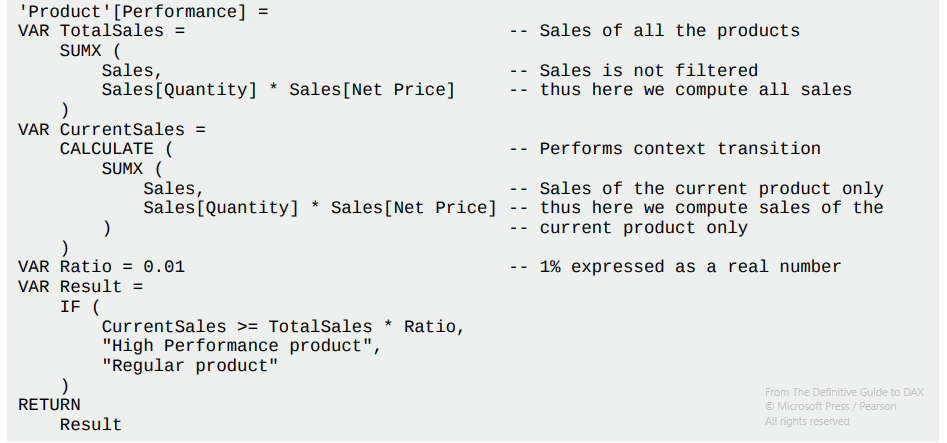
SUMX without CALCULATE ignores the row context. The solution work because the Sales column has unique IDs, so there aren’t duplicates!
Unfortunately, the CT doesn’t filter a single row but works with unique values, so we will have extremely tricky errors in case of tables with duplicates! Using this tactic is not only incorrect, but also very slow since the engine has to iterate for all the rows of the table. Using a measure is wrong too, because:
Whenever you read a measure call in DAX, you should always read it as if
CALCULATEwere there

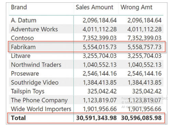
Wrong formula: the Right Sales Amount doesn’t use CALCULATE
CALCULATE modifiers (see Chapter 14)
USERELATIONSHIP, used in some edge cases (e.g. you have an Order Date and a Delivery Date, which one should you use as a Relationship Key with the Date table?). You will have to make two relationships, one active and one inactive, then add in the expressions using the inactive relationship the expressionUSERELATIONSHIP(Key1, Key2)in theCALCULATE, which tells DAX to temporarily change the status of the inactive relationship.CROSSFILTER, which is similar, but more powerful: it can disable the relationship between tables and change its direction (more on this later). I’ve never used it thoughKEEPFILTERSkeeps the existing filters likeVALUES, for example inAudio Sales KeepFilters := CALCULATE ( [Sales Amount], KEEPFILTERS ( 'Product'[Category] = "Audio" ) ). However, it doesn’t overwrite the filter context, but simply adds the filters in its arguments with anANDoperator. The outcome will then have BLANK rows if they aren’t included in the filter condition. Observe the differences:
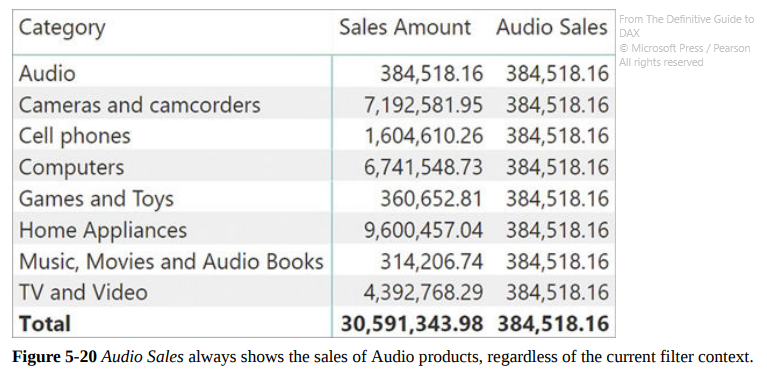
CALCULATE ( [Sales Amount], 'Product'[Category] = "Audio" )
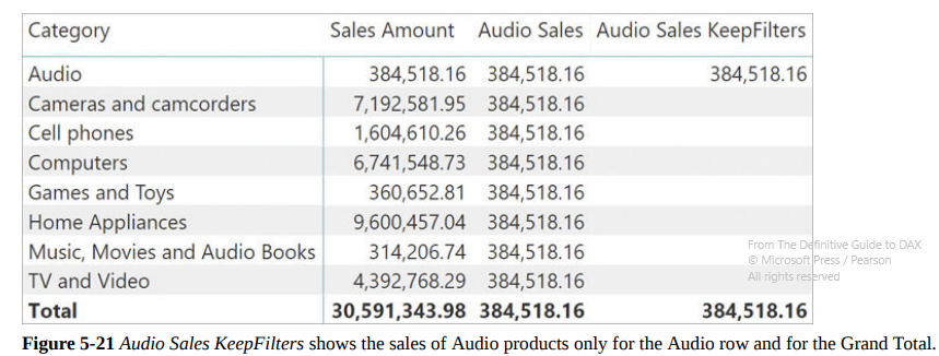
CALCULATE ( [Sales Amount], KEEPFILTERS ( 'Product'[Category] = "Audio" ) )
ALLshows a different behavior if used inside aCALCULATE, becoming a sort ofREMOVEFILTERand removing the effect of anyKEEPFILTERS, even if it’s used after the statement. That’s because the ALL* modifiers have higher execution priority than normal filters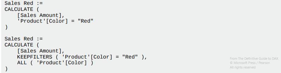 They are the same
ALLSELECTED, likeALL, has a different behavior: see Chapter 14 and be very careful when using it, it should be avoided!
6 ✨ Variables
They are important for code readability and performance optimization, use them if you see repetitions. The only thing to remember well is that they are immutable CONSTANTS calculated at the beginning of the calculation containing them. Every variables must be introduced with VAR.
Pay attention to the definition order: a variable can’t reference another variable declared later.
Another peculiarity is the name: it must be different from every existing table’s name, otherwise DAX gets confused. A best practice is to use long names precisely describing their purpose. The engine, when creating variables, uses two __as prefix
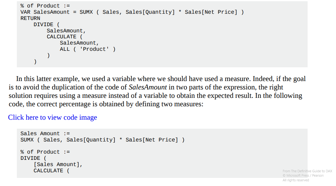 Here’s a good example about variables’ immutability
7 🔄 Working with iterators and with CALCULATE
Most of the iterators require a table and an expression used to calculate something row-by-row inside that table (e.g. SUMX calculates the sum). Specifically, the expression will iterate every row, collecting its value, then will apply the operation (in this case, a sum). Thus, all the iterators are working in the same way, except for the final operation they apply.
Keyword: iterator cardinality → it’s the number of rows scanned by the iterator and it should be kept as low as possible. You should avoid nesting different iterations, making the cardinality grow exponentially.
The chapter goes on with several interesting examples, such as how to calculate the day of the biggest sale by nesting MAXX and SUMX, or showing the list of visible colors by using CONCATENATEXeVALUES, or how ALLSELECTEDmakes more sense when used together withRANKXis the user is applying a filter, and howAVERAGEXshould be changed withDIVIDE` in case some blank values are in the data since the latter can manage automatically the division by zero and gives a correct result.
8 🔄 Time Intelligence Calculations
Very useful chapter, since dates in DAX are handled in a not-so-intuitive way.
A great tip is to always have a date table called Date in relationship with all the others for working with dates exclusively there, for optimizing performances, simply the structure and improving the user experience.
By default, PowerBI creates a hidden date table for every Time/DateTime column of the model, to create slicers and drilldowns with a calendar logic (year, quarter, month, day etc…). Unfortunately, this method creates a table for every column, causing overheads, and you can’t either view or modify them. It’s better to deactivate the automatic creation and use your user-created Date table.
Some notes
- Don’t make it huge, like 1900-2100 (ooooops 😕). It increases the cardinality and slows down calculations
- Use “ “ when mentioning the “Date” table, because
DATEis a reserved keyword in DAX (being a function) - You can quickly create your “Date” table using
CALENDARandCALENDARAUTO - Useful template from the authors: https://www.sqlbi.com/tools/dax-date-template/
- Use
USERELATIONSHIPfor making calculations with different Date columns as key (see Chapter 5 with active/inactive relationships) - DAX takes a different approach when using a Date filter in a
CALCULATEwith two columns connected with Date relationships (both keys are dates): the engine automatically addsALL (’Date’)to the formula for making possible time intelligence calculations without messing up with the context transition (see the examples) - You can apply the same special behavior with the “Mark as Date Table” command to avoid putting
ALLin every measure if you have a non-Time formatted key (e.g. int YYYYMMMDD)
Some useful functions
-
DATESYTDreturns all the dates from the beginning of the year till now, for a quick filter in aCALCULATE. There are equivalent expressions,DATESMTDandDATESQTD, for months and quarters -
Avoid the deprecated
TOTALYTD ( [Sales Amount], 'Date'[Date] ), equivalent toCALCULATE ([Sales Amount], DATESYTD(’Date’)): it has a hiddenCALCULATE! -
STARTOFYEAR, ENDOFYEAR, PREVIOUSYEAR, NEXTYEAR, DATESYTD, TOTALYTD, OPENINGBALANCEYEAR,CLOSINGBALANCEYEAR -
SAMEPERIODLASTYEARreturns a set of dates shifted one year before -
DATEADDis very powerful and flexible: you can decide how much to add (a number) and what (years, quarters, months, etc…), such asPQ Sales := CALCULATE ( [Sales Amount], DATEADD ( 'Date'[Date], -1, QUARTER ) ). It always returns days included in the Date table and it can become cumbersome during some edge cases, read well this section. -
PARALLELPERIODis useful if you are looking for the entire period despite the presence of row filters. So, for example, if you want the result of the previous quarter in the rows January, February, March writePQ Total Sales :=CALCULATE ( [Sales Amount], PARALLELPERIOD ( 'Date'[Date], -1, QUARTER ) )and see the results in the example: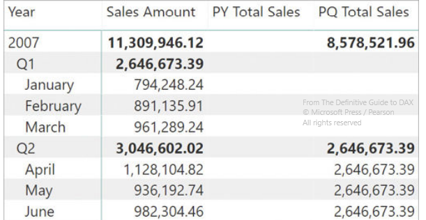
-
The functions
PREVIOUSYEAR, PREVIOUSQUARTER, PREVIOUSMONTH, PREVIOUSDAY, NEXTYEAR, NEXTQUARTER, NEXTMONTH,andNEXTDAYare using the same ‘independent’ context -
DATESINPERIODis a classic for calculating the Moving Annual Total (the total of the last 12 months). There are some alternative examples withDATESBETWEEN -
Pay attention to the semi-additive measures, which can be cumbersome. For example, a bank account balance: it’s not the sum of all the rows in the previous period, but the value at the end of the month! The suggestion is to use
LASTDATEandLASTNONBLANKto calculate the balance on the last available day, without messing up with the row context. -
STARTOFYEAR, STARTOFQUARTER, STARTOFMONTH, ENDOFYEAR, ENDOFQUARTER, ENDOFMONTHare mostly used for financial data, see the stock chart example
9 ❓ Calculations Group
They are a great way for grouping similar measures, but they currently have a great problem: they are not available on PowerBI, but you have to use the Tabular model underneath with Tabular Editor, which is a new tool. I won’t talk about them here because I found groups more complicated than useful in my case, even if I acknowledge their potentialities. Eventually, read the chapter again when you’ll notice many similar, repeated measures.
In short, instead of having many measures like
YTD Sales Amount := CALCULATE ( [Sales Amount], DATESYTD ( 'Date'[Date] ) ) YTD Total Cost := CALCULATE ( [Total Cost], DATESYTD ( 'Date'[Date] ) ) YTD Margin := CALCULATE ( [Margin], DATESYTD ( 'Date'[Date] ) )
You can create a Calculation Group, hereby called “Time Intelligence”, and use them as CALCULATE ( [Sales Amount], 'Time Intelligence'[Time calc] = "YTD" ) etc… The Time Intelligence group is like a function accepting as input parameter the field to apply to its in-memory formula. They must be simple, without aggregating different calculations. Avoid recursions and follow the best practices in the chapter’s examples. Low priority for me, as said.
10 🔄 Working with the filter context
Understanding the differences
SELECTEDVALUEvsHASONEVALUE: when using a filter, remember that filters should never return anything, but rather a default value. Use theSELECTEDVALUEshortcut, equivalent toIF(HASONEVALUE, …), that accepts a second parameter to return in case of #value != 1. To be used with slicersISFILTEREDvsISCROSSFILTERED: the first returns a boolean about the presence of filters on the table, while the latter also checks the filters on related tables that have relationships with the element passed as a parameter. In fact, if you crossfilter a column, the entire table is classified as True byISCROSSFILTERED. Remember that a table can be filtered (thusISFILTEREDgives True), yet it shows all the values (e.g. filterCustomer[City] <> "DAX”, which won’t ever happen), so treat is carefully…VALUESvsFILTERS: the first shows all the values visible in the filter context, the latter the values filtered in the filter context given as an argument. Sometimes they are the same, but if there are other active filters,VALUESmay show fewer results! I think thatFILTERSshould be used only for telling the user that at the moment he has selected those values in his slicer, or for creating tables/showing values independently from other filtersALLEXCEPTvsALL/VALUES: a classic from the book, it compares the two functions several times. They are used for selecting a single filter context from the total, usingALL(no filters)EXCEPT(filter). The first can have dangerous side effects (see Chapter 14) because it removes other filters, while a formula likeAll Values Type := CALCULATE ( [NumOfCustomers], ALL ( Customer ), VALUES ( Customer[Customer Type] ) )gives you back the ‘pure’ result, only considering the filter on the type and removing the famous context transition. Use it.ISEMPTYvsCOUNTROWS(VALUES) = 0: they are the same but the first has better performances
Data Lineage and TREATAS
Data lineage (simply explained here) is a tag that identifies the original column in the data model that we are querying. When selecting some values, PowerBI keeps some metadata, including the lineage specifying which ‘connected’ columns can be queried using the selected columns. If you use some expressions such as ADDCOLUMNS, you’ll lose the lineage, thus you will just get a raw outpout. This is important to understand for avoiding annoying side effects with filters and slicers.
E.g. having an intermediate table created manually like NewTable = {’Red’,’Blue’}, it can’t possibly know to be originated from the column Product[Color], losing all the original relationships. A slicer using NewTable won’t filter anything! With TREATAS you can forcefully assign another table’s characteristics (they must have the same structure of course!). Another good example is when you’re creating a table with custom years and you want to use it as a Date table, applying a personalized filter without iterating. Check them out.
11 ❓ Handling hierarchies
Hierarchies aren’t natively supported on DAX formulas, thus implementing them can be very tricky. A classic example is when a measure behaves differently based on the active hierarchy, for example with product categories and subcategories. In the book’s example, a combination of PercOnSubcategory := DIVIDE ( [Sales Amount], CALCULATE ( [Sales Amount], ALLSELECTED ( Product[Product Name] ) ) ) is used for calculating the percentage of each subcategory compared to all the rows of the selected category. Changing the element in the hierarchy can be done by replacing the argument in ALLSELECTED (Category, Product Name, etc…).
ISINSCOPE is a useful function that simulates a hierarchy focus, returning TRUE if the arg column is filtered and has been used for grouping (thus both row and filter contexts are using it). In the book, it is used for showing BLANK if the calculation is not about the selected hierarchy.
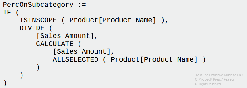

There are very advanced examples here, I wouldn’t recommend them unless they are heavily used in the current. At the moment I’m not writing down anything else.
12 🔄 Working with tables
Exploring CALCULATETABLE
A common question is about the differences between FILTER (which returns a table) and CALCULATETABLE (which is like CALCULATE but with a table). The latter is very powerful: it changes the context filter first and then calculates the expression; FILTER iterates the table and groups together the rows that are included in the filter without changing the context. You should use CALCULATETABLE whenever you want a context transition, but there’s a limit: it must be applied only on columns that belong to the data model; with measures, FILTER becomes necessary. E.g. (Large Customers = FILTER ( Customer, [Sales Amount] > 1000000)). More info about performances here.
Functions for manipulating tables
ADDCOLUMNSreturns all the rows and columns of the first parameter and adds new columns (as name, column; e.g.ColorsWithSales = ADDCOLUMNS ( VALUES ( 'Product'[Color] ), "Sales Amount", [Sales Amount] )). It’s used in complex formulas whenever creating some intermediate table, to be filtered at the end, becomes necessary.SUMMARIZEis often used for grouping values on one or more columns… A sort of GROUP BY in SQL. For example,Num of colors sold := COUNTROWS ( SUMMARIZE ( Sales, 'Product'[Color] ) )scans the Sales table and returns all the visible values there. WithVALUES, I would’ve seen ALL the colors, whether they had sales or not. Warning: do not use it alone for creating temporary columns: useADDCOLUMNS+SUMMARIZE, better optimized.CROSSJOINis like a SQL FULL JOIN, returning all the unique combinations between two tables. It seems slow and badly optimized at first, but sometimes it’s better to create a small table with all the combinations between two big tables and scan them with filters, especially when there are many duplicated values. As always, read the examples.UNIONunites all the values between two tables/columns and keeps the duplicates (useDISTINCTfor removing them); it keeps the data lineage only if both sources have the same (so, a self-JOIN): if it loses it, useTREATASfor telling the result to which column in the data model belongs.INTERSECTis the opposite: it returns the common values between two columns; less usedEXCEPTis a subtraction: it removes from the first table the rows existing in the second table
Functions for generating tables
SELECTCOLUMNSselects only the desired columns of a table: it accepts a list of column names, and it can be used when generating a new table from an existing one, usually in an intermediate step for reducing cardinality and ignoring unnecessary columns. If more than a column is passed as parameters, the data lineage is lost.ROWreturns a table with a single row. It requires a couple of names and expressions likeROW ( "Sales", [Sales Amount], "Quantity", SUM ( Sales[Quantity] ) ); it’s deprecated, just use{}DATATABLEis a more advanced table constructor; it has a more complex syntax since it requires specifying the type of each column, and you usually use it for hard-coded simple tables. I prefer making them in SQL, so I doubt I’ll use the function frequently.GENERATESERIESis like therangefunction: it returns a sequence of elements (dates, numbers) from the starting and ending parameters
13 ✨ Authoring Queries
Here we explore DAX Studio, very useful for testing, formatting and debugging DAX queries. A must-have. Since this article is becoming very long, I recommend watching some Youtube Tutorials like this one or this one to save time. It’s simpler than writing down everything that is presented in the chapter.
In short, with DAX studio you must begin your DAX scripts with the EVALUATE statement, which requires a table as the first argument (so, remember: you have to switch CALCULATE with CALCULATETABLE). With the DEFINE MEASURE keyword you can create temporary measures (which need a host table, differently from PowerBI) or variables.
DEFINE
 VAR Threshold = 200 // VAR is the same
 MEASURE Sales[LargeSales] = //LargeSales must be honested on a table like a Calculated Col
	 CALCULATE (
	 [Sales Amount],
	 Sales[Net Price] >= Threshold 	 )
EVALUATE
	ADDCOLUMNS (   // using ADDCOLUMNS because it needs a table as input
	 VALUES ( 'Product'[Category] ),
	 "Large Sales", [LargeSales]
	)
Some functions you’ll be using for authoring queries:
SUMMARIZECOLUMNS(great explanation here, a sort of LEFT JOIN) is very useful for composing a query: it requires a set of columns to group (likeSUMMARIZE), another set of columns to add to the result (likeADDCOLUMNS) and a set of filters to apply (like the extended form ofCALCULATETABLE) as arguments. It also removes blank results (bypassable withIGNORE). Its huge limitation, making it usable on DAX Studio but not on PowerBI reports, is that it becomes unusable in case of context transition, which punctually happens in charts or matrixes. It’s useful for a rapid debug though, I’ll keep it in mindTOPNis another useful expression for scripting: it returns the first N rows of a table, selecting only the columns passed as parameters. It’s useful for analyzing a new table without polluting the view with useless columns.SAMPLEis similar, but it takes the first and last rows and N rows, returning a sample of the tableISONAFTER, GENERATE, TOPNSKIP, ADDMISSINGITEMS, GROUPBY, NATURALINNERJOIN, NATURALLEFTOUTERJOIN, SUBSTITUTEWITHINDEXare functions internally used by the PowerBI engine, rarely used by a user, since there are more optimized solutions. Maybe read again their definitions if you see them in some formulas
14 🔄 Advanced DAX concepts
Expanded Tables
Expanded Tables are the core of DAX. Remember that every time you select a table, there’s a hidden world behind it that includes all its relationships!
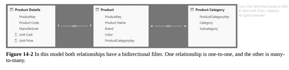
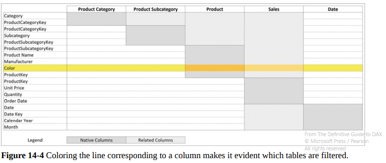
When selecting a CALCULATE filter on the Color column of Product, we can observe that the filter context uses all the linked tables, including Sales! Using RELATED, you can work on the related tables existing in the expanded table.
The ALL* functions
These functions can become extremely cumbersome, especially when used inside a CALCULATE. Pay a lot of attention to them:
ALL: it returns all of the DISTINCT values in a column/table. If used in aCALCULATEstatement, it removes any active filter, becoming a sort of REMOVEFILTER. If a column is cross-filtered it does nothingALLEXCEPT: just likeALL, but the second parameter is a list of columns that should keep their active filters. It’s slightly different from theALL/VALUEScombination (suggested by the authors): in this case,ALLremoves all filters whileVALUESkeeps the cross-filtering by adding a new filter for the visible values. On the opposite,ALLEXCEPTonly removes filtersALLNOBLANKROW: it returns all the DISTINCT values of a column/table except for, eventually, the blank rows caused by broken relationships in the data model (but not ‘normal’ blanks, blanks existing because the row just has a NULL value). If used in aCALCULATEit adds a filter for ignoring any blank in the result, which is very different!ALLSELECTED: very dangerous, it returns the distinct values in a column/table related to the latest active shadow filter. Remember that DAX has no idea about which visual/slicer the user is using on PowerBI, thusALLSELECTEDis using shadow filters behind the scenes for simulating what the user is viewing. You should never use the function in a measure that will be called by other measures, or you will cause dangerous side effects difficult to debug. Read the chapter about shadow filters for more. If used in aCALCULATEcontext, it restores the most recent shadow filter (or does nothing if there isn’t any); in the case of multiple columns, it restores a shadow filter for each parameterALLCROSSFILTERED: it doesn’t work as a table function, but only withCALCULATE, and removes every filter from the expanded table, so, every table that can be reached used the relationships of the target table. It only removes, never adds filters
Other things to remember
- Be careful with shadow filters (which work on the expanded table); they are used by
ALLSELECTand you should never touch them unless you really know what you are doing. Use column filters, and never table filters as arguments forCALCULATEexpressions for avoiding them as well - Every column of a table has its own data lineage, which is actually its representation on the data model. Whenever a filter acts, it works on the corresponding column in the model. Thus, if you lose the data lineage you won’t be able to filter. You have to use
TREATASto ‘teach’ the item about his lost position in the data model and force it back - Usually functions for grouping data keep the data lineage; filters with an aggregation generate a new one; same for
ROWandADDCOLUMNS(see examples)
15 ⚠️ Advanced Relationship
Calculated Physical Relationships
When using calculated columns for creating relationships (e.g. the DiscountDayKey calculated column, which uses Day + ProductKey in Sales for generating the % Discount with a join with the Discount table), be careful about the following details:
- Use
DISTINCTinstead ofVALUESto avoid circular dependencies - Use
ALLNOBLANKROWinstead ofALLto avoid circular dependencies (rare) - Remember that
CALCULATEwith the compact syntax hides itsFILTERand can cause circular dependencies in case of specific blanks. Use the extended version in this situation and read the examples
Virtual Relationships
Sometimes creating a relation inside the DAX query is simpler, without setting it up in the data model. It’s the same for the final user. However, they are less performant, hard to find in the codebase and more complex to handle.
There’s a nice example showing how to transfer a filter with KEEPFILTERS(TREATAS) (and maybe SUMMARIZE first for extracting the columns we need), then doing the calculations with the same filters applied on the new table; remember to use KEEPFILTERS or TREATAS will reset them!
Relationships
- SMR Single-Many Relationship
- SSR Single-Single Relationship (rare)
- MMR Many-Many Relationship (the most complex; it corresponds to two hidden bridge tables, thus it’s weak by nature and doesn’t include table expansion. Use the ‘extended form’ by creating bridge tables whenever you want to show blank values for invalid formats/relationships, otherwise they will be filtered out)
Cross-filtering gets mentioned (if a table can filter another one):
- Single: in one direction only, usually the ‘1’ in SMR can filter the ‘Many’ but not vice versa, but you can change it
- Both: both directions. It’s necessary for SSR and the default setting for MMR; be careful, because they can generate ambiguity, creating paths between tables where there shouldn’t be one.
Unless it’s necessary, try to use single relationships in the model: if you have two slicers, with a single relationship you won’t filter out the second slicer when one is active. With a ‘both’ relationship, the second element will display only the available values based on the first filter. It depends on your requirements.
Be very careful with ambiguity, it can cause nasty bugs: there could be paths between relationships (e.g. Sales → Date → Store e Sales → Ticket → Date → Store) which can become complicated with the presence of unnecessary cross-filtering. PowerBI takes the shortest road by default, but maybe that’s not what you are looking for.
16 🔄 Advanced Calculations
Short chapter with a couple of interesting use cases, I liked the first and the last the most:
- Working days between two dates: it shows some strategies like creating a boolean ‘Is Holiday’ in the Date Table and counting days while skipping the ones with ‘Is Holiday’ == False, or, for reducing iterations, groups all orders by date pairs. Read the code in the examples, you’ll learn a lot. The best solution is a calculated table with all the distinct combinations, which greatly reduces the iterations during the scanning process.
- Budget and Sales together: not useful in my situation. It creates a measure for every row with a month that shows the expected budget for the future (when Sales are still null), or the past Sales. It uses
KEEPFILTERSwith a cool trick with Max Date for reducing iterations - Computing same-store sales: not useful, the example describes a measure for considering the sales on the multi-year total only if the store was open on that specific year
- Numbering events: it can be valuable because if you try to brute-force this one you’ll have a bad time. The author wants to number the rows of a table based on the occurrences of the customer’s name (so the rows will be 1 Jon 33 EUR, 2 Jon 34 EUR, 1 Bob 2 EUR, 1 Sam 4 EUR, 2 Sam 5 EUR etc…). The right tool is
RANKXwith acustomerkey = currentCustomerKeyfilter, very effective. - Computing LY YTD: very useful, I’ve already challenged this one in the past. It uses a
TREATASto keep the data lineage, thenSAMEPERIODLASTYEAR
17 ✨ The DAX Engine
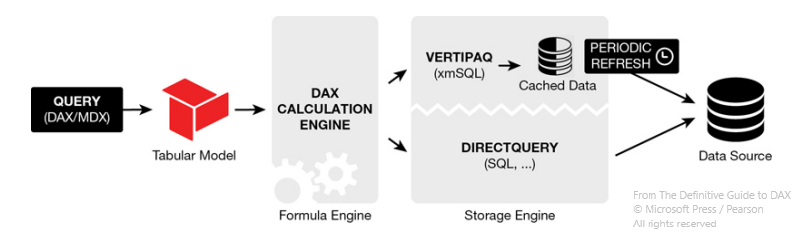
A technical segment that shows what’s happening behind the scenes. It isn’t focused on DirectQuery, which is just a SQL query translated and optimized by the Formula Engine, but rather on VertiPaq, which uses an in-memory copy of the table which will be queried by the Formula Engine too (it doesn’t work with uncompressed tables).
A third query mode can be Dual, with a table read in-memory during data refresh, but read with DirectQuery at query time.
VertiPaq is a columnar database, very effective when you want to filter many rows on a few columns, but slower when filtering a few rows on many columns. Its structure is a transposition of a classic database. Its objective is to be as efficient as possible by compressing data with several methods: hash encryption, unit encoding, RLE, intermediate tables and so on…
Optimization
You have to keep in mind only one thing from this section: the performance cost of a relationship depends on the cardinality (the number of unique values) of the columns used in the relationship. Over 100k unique values the delay becomes noticeable, so pay attention when using RELATED or cross-filtering different tables.
Materialization
It’s a step in the query execution process used with columnar DBs. Every time the formula engine makes a request, it receives back a temporary table called datacache; it’s a materialization that will be consumed in both cases: DirectQuery or VertiPaq. It’s the engine’s way to get access to raw data. If the datacache has the same cardinality of the final result it’s considered ‘late’ (very rare for complex calculations), otherwise, it will be ‘early’. Just remember that datacaches are intermediate data between the raw DB query in SQL and the processing engines.
Aggregation
It’s an engine trick for optimizing the storage engine queries by using group by clauses. The most common aggregations are already included in the tables, ready to be used.
Furthermore, there are details about the Hardware, not interesting in my case.
18 ❓ Optimizing VertiPaq
The book introduces DVM, with several examples for monitoring every table’s size and relationships. I will not go into it further.
Denormalization
Every relationship has a memory cost. VertiPaq tries to denormalize unused tables, reducing their column and relationships. There could be problems (technical problems) when this clashes with another tendency of VertiPaq: normalizing everything for speeding up operations and creating tons of intermediate tables. Eventually, the book suggests forcefully creating inactive/active relationships ‘forcing’ the engine to denormalize some tables/columns and avoiding performance issues. I didn’t understand this part well, honestly.
Cardinality
As said before, it’s the number of unique values that a column contains; it’s an important measure for calculating the size of the column, which will in turn impacts the VertiPaq performances. Here are some tricks for reducing cardinality:
- Round floats whenever possible
- For images: store a URL string, PowerBI can’t process plain images
- Transactions IDS: they are unique values, causing max cardinality, but are rarely used. Take them away
- Date and Time: it’s better to split the Date column into two: a Date (with days only) and Time (with values from 00.00 to 23.59): there are some example scripts, reducing the cardinality of the Date table by A LOT. It’s a great way to optimize a model
- Audit columns: they are rarely used (such as ‘last edited’ and ‘last edited by’), don’t import them
Calculated Columns
They can be useful for optimization since they are evaluated row-by-row after a table refresh, but it’s always the case. Predicting if the performance will be better or worse is difficult because calculated columns aren’t as optimized as the ‘normal’ columns on the DB. You have to try and compare the outputs. Usually, they are suggested when filtering and grouping data, and when considering boolean types.
Remember that unnecessary ID columns that aren’t used in the model have the highest cardinality and are just slowing down the model. Prioritize qualitative columns (such as category or date range) and import quantitative columns, which often have high cardinality, only if necessary.
19 🔄 Analyzing DAX Queries
With DAX Studio it is possible to analyze all the queries we are making through PowerBI and recognize the slower ones. It’s shown that the Formula Engine creates a Logical Tree (by translating DAX into instructions) and then a Physical Tree (lower level instructions for the machine)
Plans
- DAX

- Logical Query Plan: it’s still easy to trace back its relationship with the original DAX version. In this case, it corresponds to “Create a table with a column named Value, filled with the content of a SUM operation, performed by the storage engine by scanning the Quantity column in the Sales table.”

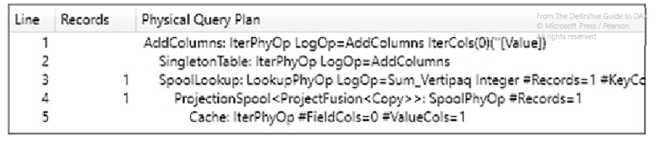
- Physical Query Plan: it looks similar to the Logical Tree, but it goes deeper, with different operators and a more complex structure, difficult to interpret. Some important details are hidden here though! Pay attention to ProjectionSpool, which shows the number of records picked up by the engine from the DB with a SQL query. Being the step a single thread and using memory, it could be a bottleneck
- the XmSQL query generated by the Storage Engine’s ProjectionSpool, which is what the database will receive as input. This is just the SQL conversion of the previous step, you can’t intervene
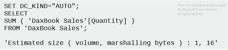
Then, there are some technicalities about xmSQL, not really my cup of tea. Just a final reminder: remember to clean up the cache before analyzing performances, since the engine stores previous datacaches in memory and the processing speed will be faster than in reality.
CallbackDataId
If in the DAX formula there are complex elements such as IF or SQRT, then the Formula Engine will insert in its XmSQL query plan the CallbackDataId statement. E.g. for a ROUND, there will be something like
WITH
$Expr0 := [CallbackDataID ( ROUND ( Sales[Line Amount]] ), 0 ) ]
( PFDATAID ( Sales[Line Amount] ) )
SELECT
SUM ( @$Expr0 )
FROM Sales;
These calls are more expensive and they can’t be stored in the cache. Knowing that you can optimize some measures by using simple elements, like replacing a IF denominator != 0statement with a SUMX + FILTER (denominator <> 0). Yeah, just avoid IFs if you can. Of course, sometimes CallbackDataID must be used, there’s no problem… Just be aware of that
20 ❓ Optimizing DAX
Last chapter with some ideas for speeding up executions, but it really depends on the data underneath so these aren’t fixed rules. Try every solution before accepting it.
The optimization process in DAX is:
- Identify a SINGLE query in DAX. With complex formulas, try to break them down into smaller steps (well commented)
- Create a query in DAX Studio simulating the selected step. Use
EVALUATEandCALCULATE(TABLE)as we have seen in Chapter 13. DAX Studio has a “Define Measure” button that already creates a query in the lateral panel, check it out! - Analyze the execution times of the server and the information in the query plan
- Identify bottlenecks in both SE and FE. For example, if %SE >> %FE something’s wrong with the DAX formula. Start from the Storage Engine queries (both Physical and Logical) and see how many records are picking up
- Implement changes and re-run the query to observe if the performances have improved
Optimizing DAX expressions
Usually, the causes of long runtimes of a DAX formula are:
- Longer scan times: cardinality matters here: the more unique values you have, the more time the scanning operators need
- High Cardinality: same. It will be an issue for
COUNTandCALCULATE’s filters in particular - High presence of CallbackDataID: remember to use simple operators if you can
- Large Materialization: if the datacache is large, more RAM will be needed. Usually, this depends on the size of the data you want to analyze
Tips
- Optimizing filters: in
CALCULATEstatements, the filter parameter must act on columns and not on entire tables (avoiding both the use of shadow filters and storing the whole table in memory). You should use aKEEPFILTERSinstead for keeping the current filters and then selecting just the columns you want - Optimizing context transition: this is more complex, please read the example. Here, instead of using a
SUMXoverCustomers, Sales Amount x Cashback %, the book usesSUMXoverVALUES(Customer[Cashback%], Sales Amount x Cashback %. By just usingVALUESand selecting only the visible cashback in the current filters, there is a smaller datacache in memory and a faster query. Otherwise, the default strategy would have been of calculating the cashback for every combination of customerKey in the table, and then filter - Optimizing
IFconditions:IFs are slow because they always need a CallbackDataID, and this can slow the query down, especially when multiple conditional checks happen for every row. Avoid them by using aCALCULATE+KEEPFILTERSstatement during some edge cases (see example) - Choose between
IFandDIVIDE: already mentioned before. For divisions, where you don’t want errors in the case of denominators == 0, useDIVIDEinstead of anIFstatement because the first is way better optimized - Optimizing
IFin iterators: another strategy for avoiding slowdowns with conditional statements and iterations is to use twoCALCULATEwith filters. Again, see the example, sometimes this strategy can be slow, but it’s easily scalable - Reducing the use of CallbackDataID: this is very nice; you can replace
SUMX(Sales, Sales[Quantity] * ROUND(Sales[Net Price],0))withSUMX(VALUES(Sales[Net Price], CALCULATE(SUM(Sales[Quantity]) * ROUND(Sales[Net Price]0)and the engine will store part of the query in memory, speeding up future operations! Then CallbackDataID will be used for the second part, but at least it’s an improvement. Be careful that if Net Price has high cardinality the trick is useless - Avoid table filters for
DISTINCTCOUNT: if used with aCALCULATEand a filter on, say, the Sales table, it will apply a query for each product! Slow, veeeery slow! The optimized version usesKEEPFILTERS(FILTER(ALL(Sales[Quantity], Sales[Net Price]), *your_filters)